Adding Geospatial Features to Your Machine Learning Models
Published:
Introduction
When we build machine learning models, we often focus on features like numbers, categories, and texts. But there’s one feature type that often gets ignored: location.
And that’s a problem, because location is more than just a pair of coordinates - it carries context. For example:
- Two houses with the same number of rooms can have very different prices depending on how close they are to the city center.
- A restaurant’s success depends not only on its menu, but also on the number of offices or schools around it.
- Crop yield is influenced not just by fertilizer, but by soil type, elevation, and distance to rivers.
In other words, location shapes outcomes. The good news is: adding location is easier than you think.
In this hands-on tutorial, we’ll walk through building a location-aware machine learning model using Airbnb data from New York City. This model can predict the price of an Airbnb listing.
Setting up the Environment
Before working with the dataset, it’s important to set up the right environment. In this project, we’ll combine Python’s data science and geospatial analysis ecosystem. The toolkit includes core libraries such as pandas for data handling, geopandas (an extension of pandas for spatial data), shapely for geometric operations, and scikit-learn for machine learning. For mapping and data access, we’ll rely on folium to create interactive maps and osmnx to seamlessly download data from OpenStreetMap.
# !pip install pandas geopandas shapely scikit-learn folium osmnx
import pandas as pd
import geopandas as gpd
import shapely
import sklearn
import folium
import osmnx as ox

print("All libraries loaded successfully!")
All libraries loaded successfully!
If that runs without errors, you’re ready to go.
Dataset Preparation
Now that our environment is ready, let’s load some real-world data. For this tutorial, we’ll use the Inside Airbnb dataset for New York City. This dataset is public and widely used by researchers, making it a great starting point.
About the dataset
The Airbnb NYC dataset includes:
- Basic info about listings (price, room_type, number_of_reviews, availability…).
- Location info (latitude and longitude).
- Neighborhood details.
Download dataset
You can grab the dataset directly from Inside Airbnb (https://insideairbnb.com/get-the-data/) and look for: New York City, Detailed Listing data (CSV).
Load data in Python
import pandas as pd

df = pd.read_csv("./data/listings.csv")

df.head(3)
| id | listing_url | scrape_id | last_scraped | source | name | description | neighborhood_overview | picture_url | host_id | ... | review_scores_communication | review_scores_location | review_scores_value | license | instant_bookable | calculated_host_listings_count | calculated_host_listings_count_entire_homes | calculated_host_listings_count_private_rooms | calculated_host_listings_count_shared_rooms | reviews_per_month | |
|---|---|---|---|---|---|---|---|---|---|---|---|---|---|---|---|---|---|---|---|---|---|
| 0 | 2539 | https://www.airbnb.com/rooms/2539 | 20250801203054 | 2025-08-03 | city scrape | Superfast Wi-Fi. Clean & quiet home by the park | Bright, serene room in a renovated apartment h... | Close to Prospect Park and Historic Ditmas Park | https://a0.muscache.com/pictures/hosting/Hosti... | 2787 | ... | 5.0 | 4.75 | 4.88 | NaN | f | 6 | 1 | 5 | 0 | 0.08 |
| 1 | 2595 | https://www.airbnb.com/rooms/2595 | 20250801203054 | 2025-08-02 | city scrape | Skylit Studio Oasis | Midtown Manhattan | Prime Midtown | Spacious 500 Sq Ft | Pyramid S... | Centrally located in the heart of Manhattan ju... | https://a0.muscache.com/pictures/hosting/Hosti... | 2845 | ... | 4.8 | 4.81 | 4.40 | NaN | f | 3 | 3 | 0 | 0 | 0.25 |
| 2 | 6848 | https://www.airbnb.com/rooms/6848 | 20250801203054 | 2025-08-03 | city scrape | Only 2 stops to Manhattan studio | Comfortable studio apartment with super comfor... | NaN | https://a0.muscache.com/pictures/e4f031a7-f146... | 15991 | ... | 4.8 | 4.69 | 4.58 | NaN | f | 1 | 1 | 0 | 0 | 0.99 |
3 rows × 79 columns
Turn it into a GeoDataFrame
Since we’ll be working with spatial features, let’s convert it into a GeoDataFrame using geopandas:
import geopandas as gpd
from shapely.geometry import Point

gdf = gpd.GeoDataFrame(
	df,
	geometry=gpd.points_from_xy(df.longitude, df.latitude),
	crs="EPSG:4326"
)

gdf.head(3)
| id | listing_url | scrape_id | last_scraped | source | name | description | neighborhood_overview | picture_url | host_id | ... | review_scores_location | review_scores_value | license | instant_bookable | calculated_host_listings_count | calculated_host_listings_count_entire_homes | calculated_host_listings_count_private_rooms | calculated_host_listings_count_shared_rooms | reviews_per_month | geometry | |
|---|---|---|---|---|---|---|---|---|---|---|---|---|---|---|---|---|---|---|---|---|---|
| 0 | 2539 | https://www.airbnb.com/rooms/2539 | 20250801203054 | 2025-08-03 | city scrape | Superfast Wi-Fi. Clean & quiet home by the park | Bright, serene room in a renovated apartment h... | Close to Prospect Park and Historic Ditmas Park | https://a0.muscache.com/pictures/hosting/Hosti... | 2787 | ... | 4.75 | 4.88 | NaN | f | 6 | 1 | 5 | 0 | 0.08 | POINT (-73.97238 40.64529) |
| 1 | 2595 | https://www.airbnb.com/rooms/2595 | 20250801203054 | 2025-08-02 | city scrape | Skylit Studio Oasis | Midtown Manhattan | Prime Midtown | Spacious 500 Sq Ft | Pyramid S... | Centrally located in the heart of Manhattan ju... | https://a0.muscache.com/pictures/hosting/Hosti... | 2845 | ... | 4.81 | 4.40 | NaN | f | 3 | 3 | 0 | 0 | 0.25 | POINT (-73.98559 40.75356) |
| 2 | 6848 | https://www.airbnb.com/rooms/6848 | 20250801203054 | 2025-08-03 | city scrape | Only 2 stops to Manhattan studio | Comfortable studio apartment with super comfor... | NaN | https://a0.muscache.com/pictures/e4f031a7-f146... | 15991 | ... | 4.69 | 4.58 | NaN | f | 1 | 1 | 0 | 0 | 0.99 | POINT (-73.95342 40.70935) |
3 rows × 80 columns
Quick Visualization
Let’s quickly check where the listings are located on a map:
import folium

# Pick a center (Manhattan coordinates)
m = folium.Map(location=[40.75, -73.98], zoom_start=11)

for idx, row in gdf.head(500).iterrows():
	folium.CircleMarker([row.latitude, row.longitude], radius=2, color="red", fill=True).add_to(m)

m
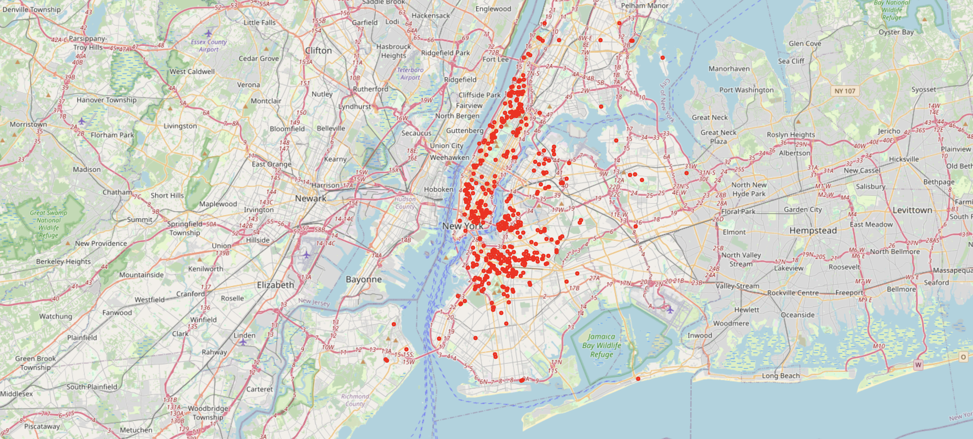
You should see an interactive map with points spread across New York’s boroughs.
Feature Engineering with Location
Although our dataset knows where each Airbnb is located, raw latitude/longitude numbers don’t mean much for a machine learning model. We need to transform location into features that capture geographic context. Here are four useful and simple types of location-based features we’ll create.
1. Distance to the City Center
Why it matters: in most cities, listings closer to the city center tend to be more expensive. Proximity to central business districts often reflects accessibility, demand, and prestige.
from shapely.geometry import Point

# Define the city center (Times Square)
city_center = Point(-73.9855, 40.7580)

# Computer distance
gdf = gdf.to_crs(epsg=3857) # Project to metric system
gdf['dist_city_center'] = gdf.geometry.distance(city_center)
gdf[['neighbourhood_group_cleansed', 'price', 'dist_city_center']].head(3)
| neighbourhood_group_cleansed | price | dist_city_center | |
|---|---|---|---|
| 0 | Brooklyn | $260.00 | 9.612996e+06 |
| 1 | Manhattan | $240.00 | 9.622467e+06 |
| 2 | Brooklyn | $98.00 | 9.616044e+06 |
2. Distance to the Nearest Park
People love staying near green spaces - parks improve livability, reduce noise, and offer recreation.
import osmnx as ox

# Get all paarks in NYC from OpenStreetMap
tags = {'leisure': 'park'}
parks = ox.features_from_place("New York City, USA", tags)

# Convert to centroids
parks = parks.to_crs(epsg=3857).centroid

# Computer nearest park distance
gdf['dist_nearest_park'] = gdf.geometry.apply(lambda x: parks.distance(x).min())
3. Distance to the Nearest Subway Station
In New York, proximity to the subway is a huge factor. It can make or break the attractiveness of a listing. This is where location truly shines - coordinates alone don’t tell you if there’s a subway nearby.
tags = {"railway": "station", "station": "subway"}
subways = ox.features_from_place("New York City, USA", tags)

subways = subways.to_crs(epsg=3857).centroid

gdf['dist_nearest_subway'] = gdf.geometry.apply(lambda x: subways.distance(x).min())

gdf[['neighbourhood_group_cleansed', 'price', 'dist_city_center', 'dist_nearest_park', 'dist_nearest_subway']].head(3)
| neighbourhood_group_cleansed | price | dist_city_center | dist_nearest_park | dist_nearest_subway | |
|---|---|---|---|---|---|
| 0 | Brooklyn | $260.00 | 9.612996e+06 | 695.029979 | 832.818934 |
| 1 | Manhattan | $240.00 | 9.622467e+06 | 190.688019 | 149.614085 |
| 2 | Brooklyn | $98.00 | 9.616044e+06 | 272.811822 | 366.446845 |
4. Neighborhood Density
Density captures how “crowded” an area is. A high density might signal popularity (lots of demand) but also strong competition.
from sklearn.neighbors import BallTree
import numpy as np

# Extract coordinates in radians
coords = np.vstack([gdf.geometry.y, gdf.geometry.x]).T
coords_rad = np.radians(coords)

tree = BallTree(coords_rad, metric="haversine")

# Count neighbors within 1 km
neighbors_count = tree.query_radius(coords_rad, r=1000/6371000, count_only=True)
gdf['density_1km'] = neighbors_count

gdf[['neighbourhood_group_cleansed', 'price', 'dist_city_center', 'dist_nearest_park', 'density_1km']].head(3)
| neighbourhood_group_cleansed | price | dist_city_center | dist_nearest_park | density_1km | |
|---|---|---|---|---|---|
| 0 | Brooklyn | $260.00 | 9.612996e+06 | 695.029979 | 1 |
| 1 | Manhattan | $240.00 | 9.622467e+06 | 190.688019 | 1 |
| 2 | Brooklyn | $98.00 | 9.616044e+06 | 272.811822 | 1 |
Our Location Features
At this point, our dataset has four new features:
- dist_city_center → Accessibility to Manhattan’s core
- dist_nearest_park → Environmental quality
- density_1km → Neighborhood competition/attractiveness
- dist_nearest_subway → Transportation accessibility
Together, these features show why location is more than just lat/long. They turn spatial context into measurable signals that our model can actually use.
✅ With this enriched dataset, we’re ready for the fun part: training two models — one without location features, and one with them — and seeing how much location improves predictions.
Training the Model
📊 Baseline model (without location)
For the baseline, we’ll use only non-spatial attributes:
- room_type
- minimum_nights
- number_of_reviews
- availability_365
We will predict the price of a listing.
from sklearn.model_selection import train_test_split
from sklearn.ensemble import RandomForestRegressor
from sklearn.metrics import mean_absolute_error, r2_score

# Select baseline features
baseline_features = ["room_type", "minimum_nights", "number_of_reviews", "availability_365"]

gdf['price'] = gdf['price'].astype(str).str.replace("$", "", regex=False)
gdf['price'] = gdf['price'].astype(str).str.replace(",", "", regex=False)
gdf['price'] = gdf['price'].astype(float)
gdf = gdf[gdf['price'].notna()]

# Encode categorical variable (room_type)
df_encoded = pd.get_dummies(gdf[baseline_features + ["price"]], drop_first=True)
X = df_encoded.drop("price", axis=1)
y = df_encoded["price"]

# Train/test split
X_train, X_test, y_train, y_test = train_test_split(X, y, test_size=0.2, random_state=42)

# Train baseline model
baseline_model = RandomForestRegressor(n_estimators=100, random_state=42)
baseline_model.fit(X_train, y_train)

# Predictions
y_pred_baseline = baseline_model.predict(X_test)

# Evaluate
print("Baseline MAE: ", mean_absolute_error(y_test, y_pred_baseline))
Baseline MAE: 219.09178855984604
🌍 Location-Aware Model (With spatial features)
Now let’s add our geographic features:
- dist_city_center
- dist_nearest_park
- dist_nearest_subway
- density_1km
# Select both baseline + spatial features
spatial_features = baseline_features + ["dist_city_center", "dist_nearest_park", "dist_nearest_subway", "density_1km"]

df_encoded_spatial = pd.get_dummies(gdf[spatial_features + ["price"]], drop_first=True)

X2 = df_encoded_spatial.drop("price", axis=1)
y2 = df_encoded_spatial["price"]

# Train/test split
X2_train, X2_test, y2_train, y2_test = train_test_split(X2, y2, test_size=0.2, random_state=42)

# train location-aware model
spatial_model = RandomForestRegressor(n_estimators=100, random_state=42)
spatial_model.fit(X2_train, y2_train)

# Prediction
y_pred_spatial = spatial_model.predict(X2_test)

# Evaluate
print("Location-Aware MAE: ", mean_absolute_error(y2_test, y_pred_spatial))
Location-Aware MAE: 205.12980100334863
At this point, the location-aware model outperforms the baseline. The MAE of the location-aware model is lower than the baseline -> the predictions are closer to the real price than the prediction without using spatial features.
Evaluating and Visualizing Results
Feature Importance
import matplotlib.pyplot as plt
import seaborn as sns

importances = spatial_model.feature_importances_
features = X2_train.columns
feat_imp = pd.Series(importances, index=features).sort_values(ascending=False)

plt.figure(figsize=(8,5))
sns.barplot(x=feat_imp.values, y=feat_imp.index)
plt.title("Feature Importance (Location-Aware Model)")
plt.show()
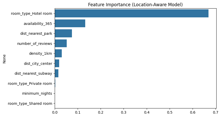
This feature importance plot for our location-aware Airbnb price prediction model reveals the key drivers behind listing prices. Strikingly, the room_type feature stands out as overwhelmingly the most influential, suggesting that properties classified as hotel rooms have a distinct pricing structure that significantly impacts the model’s predictions.
Following this, availability_365 and dist_nearest_park emerge as the next most significant factors. The importance of proximity to parks highlights how granular local amenities contribute to pricing, often more so than just a general dist_city_center. Other location-based features like density_1km and dist_nearest_subway also play their part, affirming the value of our location-aware approach.
Visualizing results
Numbers are good, but maps make results tangible. Let’s map predicted prices from the location-aware model vs. the actual prices.
import folium
import warnings
warnings.filterwarnings("ignore")

features_encoded = df_encoded_spatial.columns.to_list()
features_encoded.remove("price")

gdf_encoded = pd.get_dummies(gdf[spatial_features + ["price"]], drop_first=True)
gdf_encoded['latitude'] = gdf['latitude']
gdf_encoded['longitude'] = gdf['longitude']

# Create base map
m = folium.Map(location=[40.73, -73.93], zoom_start=11)

# Add predicted values as circle markers
for _, row in gdf_encoded.sample(500).iterrows():
	folium.CircleMarker(
		location=[row.latitude, row.longitude],
		radius=4,
		popup=f"Actual: ${row['price']} | Predicted: ${spatial_model.predict([row[features_encoded].values])[0]:.0f}",
		color="blue",
		fill=True,
		fill_opacity=0.6
	).add_to(m)

m.save("outputs/airbnb_predictions_map.html")
This lets us:
- Spot over- or under-valued areas (e.g., overpriced listings in less central areas).
- Show how predictions vary spatially, rather than just as numbers.
- Engage readers with an interactive, reality-grounded view.
GeoAI is not only about better accuracy, but also about better understanding.
Conclusion
In this blog, we built two machine learning models to predict Airbnb prices: one with standard features and another with added spatial context. The location-aware model outperformed the baseline, and the location-aware approach also highlighted something equally valuable: a property’s location shapes its value.
By engineering and analyzing spatial features, we saw how distance to the city center, nearby amenities, and neighborhood density influence pricing patterns. Beyond accuracy, this experiment shows that GeoAI isn’t just about building stronger models — it’s about adding a layer of geographic understanding that helps us interpret real-world dynamics.
Author: Felix Do